Binomial Distribution

Binomial Distribution for Successive Events

An experiment may be repeated n times and each of these n trials are independent of one another. If each trial only gives one of the two possible outcomes, say 'success' (when required event take place) and failure (when required event does not take place) then it is called a Binomial Experiment. Let probability of success in any trial be p and that of failure be q, then
p + q = 1

Then (p + q)ⁿ = C₀ Pⁿ + C₁P^n-1q +...... C_rp^n-rq^r +...+ C_nqⁿ

Then the probability of exactly k successes in n trials is given by

P_k = ⁿC_kq^n-kp^k

A binomial distribution can also be defined as the distribution that describes the behavior of a count variable X satisfying the following conditions:

1: The number of observations n is fixed.

2: Each observation is independent.

3: Each observation represents one of two outcomes ("success" or "failure").

4: The probability of "success" p is the same for each outcome.

If these conditions are met, then X has a binomial distribution with parameters n and p, abbreviated B (n,p).

Some important facts related to binomial distribution:

(i)                The probability of getting at least k successes is

           P(x > k) = Σⁿ_x=k  ⁿC_x p^x q^n-x

(ii)    Σⁿ_x=k  ⁿC_x q^n-x p^x = (q + p)ⁿ = 1.

(iii) Mean of binomial distribution is np,

(iv) Variance is npq,

(v) Standard deviation is given by (npq)^1/2, where n,p and q have their meanings as described above.

Example: Suppose individuals with a certain gene have a 0.70 probability of eventually contracting a certain disease. If 100 individuals with the gene participate in a lifetime study, then the distribution of the random variable describing the number of individuals who will contract the disease is distributed B(100,0.7).

Note: The Binomial distribution is only apt in cases where the population size is significantly larger than the sample size. So, in general the binomial distribution should not be applied to observations unless the population size is at least 10 times larger than the sample size.

Illustration:

What is the probability of getting exactly 2 heads in 6 tosses of a fair coin?

Solution:

This is clearly a question of binomial distribution and hence substituting the values of x as 2 and of n as 6 we get

P(X = 2) = 6! / (2! 4!) (1/2)² (1/2)^6-2 = 15/64

Illustration:

A survey from Teenage Research Unlimited (Northbrook, Ill.) found that 30% of teenage consumers receive their spending money from part-time jobs.  If five teenagers are selected at random, find the probability that at least three of them will have part-time jobs.

 Solution:

To find the probability that at least three have a part-time job, it is necessary to find the individual probabilities for 3, 4, or 5 and then add them to get the total probability.


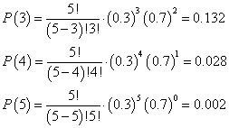
Hence,

    P (at least three teenagers have part-time jobs) = 0.132 + 0.028 + 0.002 = 0.162

Illustration:

In a rainy season, there is 60% chance that it will rain on a particular day. What is the probability that there will be exactly 4 rainy days in a week?

Solution:

Let probability of raining on a particular day p (success) = 3/5

And probability that no rain occurs on a particular day q (failure) = 2/5

Probability of exactly 4 rainy days i.e. 4 successes out of 7 trials

= ⁷C₄ (p)⁴(q)³ =  ( 7!/4!.3! ) * (3/5)⁴ * (2/5)³

Illustration:

If a student randomly guesses at five multiple-choice questions, find the probability that the student gets exactly three correct.  Each question has five possible choices.

Solution:

In this case n = 5, X = 3, and p = 1/5, since there is one chance in five of guessing a correct answer.  Then,

P (3) = 5! / (5-3)! 3! (1/5)³(4/5)² = 0.05.

For more examples you may view the video

Sums of binomials

If X ~ B(n, p) and Y ~ B(m, p) are independent binomial variables with the same probability p, then X + Y is again a binomial variable; its distribution is

X + Y ~ B( n+m, p).

Conditional binomials

If X ~ B(n, p) and, conditional on X, Y ~ B(X, q), then Y is a simple binomial variable with distribution

Y ~ B( n, pq).

Bernoulli distribution

The Bernoulli distribution is a special case of the binomial distribution, where n = 1. Symbolically, X ~ B (1, p) has the same meaning as X ~ Bern (p). Conversely, any binomial distribution, B (n, p), is the distribution of the sum of n independent Bernoulli trials Bern (p), each with the same probability p.

Poisson binomial distribution

The binomial distribution is a special case of the Poisson Binomial Distribution which is a sum of n independent non-identical Bernoulli trials Bern(p_i).  If X has the Poisson binomial distribution with p₁ = … = p_n =p then X ~ B(n, p).

You may consult the Sample Papers to get an idea about the types of questions asked.

Cumulative Binomial Probability

A cumulative binomial probability refers to the probability that the binomial random variable falls within a specified range (e.g., is greater than or equal to a stated lower limit and less than or equal to a stated upper limit).

For instance consider the cumulative binomial probability of obtaining 45 or fewer heads in 100 tosses of a coin. This would be the sum of all these individual binomial probabilities.

b(x < 45; 100, 0.5) =
b(x = 0; 100, 0.5) + b(x = 1; 100, 0.5) + ... + b(x = 44; 100, 0.5) + b(x = 45; 100, 0.5)

Illustration:

The probability that a student is accepted to a prestigious college is 0.3. If 5 students from the same school apply, what is the probability that at most 2 are accepted?

Solution:

To solve this problem, we compute 3 individual probabilities, using the binomial formula. The sum of all these probabilities is the required answer. Thus,

b(x < 2; 5, 0.3) = b(x = 0; 5, 0.3) + b(x = 1; 5, 0.3) + b(x = 2; 5, 0.3)
b(x < 2; 5, 0.3) = 0.1681 + 0.3601 + 0.3087
b(x < 2; 5, 0.3) = 0.8369

Negative Binomial distribution: We first discuss negative binomial experiment and then proceed towards negative binomial distribution.

A negative binomial experiment is an experiment which consists of x repeated trials in which each trial can result in just two possible outcomes a success or a failure. In addition to this it has the following properties:

• The probability of success, denoted by P, is the same on every trial.

• The trials are independent; that is, the outcome on one trial does not affect the outcome on other trials.

• The experiment continues until r successes are observed, where r is specified in advance.

In order to clarify this we consider an experiment of flipping a coin repeatedly and count the number of times the coin lands on heads. You continue flipping the coin until it has landed 5 times on heads. This is a negative binomial experiment because:

• The experiment consists of repeated trials. We flip a coin repeatedly until it has landed 5 times on heads.

• Each trial can result in just two possible outcomes - heads or tails.

• The probability of success is constant - 0.5 on every trial.

• The trials are independent; that is, getting heads on one trial does not affect whether we get heads on other trials.

• The experiment continues until a fixed number of successes have occurred; in this case, 5 heads.

Negative Binomial Distribution

A negative binomial random variable is the number X of repeated trials to produce r successes in a negative binomial experiment. The probability distribution of this random variable is called the negative binomial distribution.

Again consider the case of flipping a coin repeatedly and count the number of heads (successes). If we continue flipping the coin until it has landed 2 times on heads, we are conducting a negative binomial experiment. The negative binomial random variable is the number of coin flips required to achieve 2 heads. Hence in this case the random variable is the number of coin flips that can take on any integer value between 2 and plus infinity. The negative binomial probability distribution for this example is presented below.

Number of coin flips      Probability

                  2                         0.25

                  3                         0.25

                  4                         0.1875

                  5                         0.125

                  6                         0.078125        

           7 or more                 0.109375

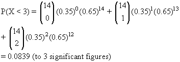
Illustration:

The probability that sixth formers know what the first prime number is, is 0.35.

Find the probability that in a sample of 14 sixth formers, the numbers who know is...

1. exactly 3;

2. less than 3, and;

3. greater than 1.

If we let X be the number of successes, our distribution is given by:

X~ B(14,0.35)

Using the formula:

P(X=r) = ⁿC_r p^rq^n-r

Therefore P(x=3) = 364 (0.35)³ (0.65)¹¹

= 0.137

Therefore:

To get P(X > 1), we could calculate this by working out: P(X = 2) + P(X = 3) + P(X = 4)... + P(X = 14), taking a very long time! Instead, we use the fact that these distributions sum to 1 (they are exhaustive!)

Therefore:



Binomial Distribution is an important topic in the Mathematics syllabus of the IIT JEE. It is vital to master this topic to remain competitive in the JEE.

To read more, Buy study materials of Probability comprising study notes, revision notes, video lectures, previous year solved questions etc. Also browse for more study materials on Mathematics here.