

Adsorption is often used as a polishing step to provide advanced treatment for hardly degradable substances present in secondary effluents. An activated was obtained and batch adsorption experiments were carried out to establish adsorption isotherm for the carbon. The data given in Table 1 represent equilibrium chlorbbenzene (CB) concentrątionş obtained in batch adsorption experiments where 1 g of activated carbon was added into each of seven beakers containing 1 liter of wastewater with varying initial chlorobenzene concentrątion.Given:Contaminant = chlorobenzene [C6H5CL] (CB)BC Saturation concentration = 500 mg/L - Derive the adsorption constants using the
a) Freundlich model b) Langmuir model c) BET model Use a spreadsheet to analyze the datá and establish which model describes best adsorption on the given carbon and why? Tabulate your answers of experimental constants for each model along with the appropriate regression parameter - Based on the analysis above which carbon would you recommend for effective removal of chlorobenzene and why?
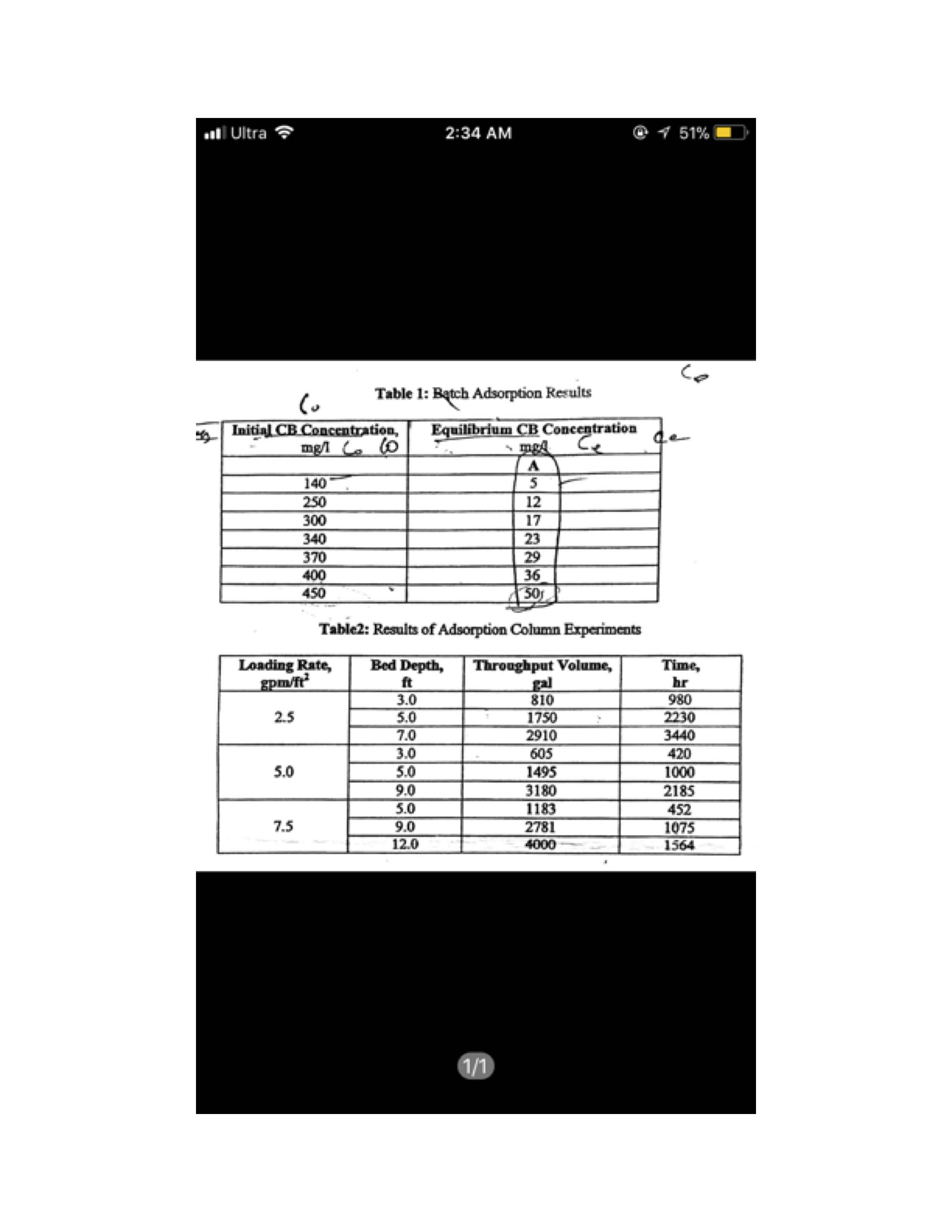
Adsorption is often used as a polishing step to provide advanced treatment for hardly degradable substances present in secondary effluents. An activated was obtained and batch adsorption experiments were carried out to establish adsorption isotherm for the carbon. The data given in Table 1 represent equilibrium chlorbbenzene (CB) concentrątionş obtained in batch adsorption experiments where 1 g of activated carbon was added into each of seven beakers containing 1 liter of wastewater with varying initial chlorobenzene concentrątion.
Given:
Contaminant = chlorobenzene [C6H5CL] (CB)
BC Saturation concentration = 500 mg/L
- Derive the adsorption constants using the
a) Freundlich model
b) Langmuir model
c) BET model
Use a spreadsheet to analyze the datá and establish which model describes best adsorption on the given carbon and why? Tabulate your answers of experimental constants for each model along with the appropriate regression parameter
- Based on the analysis above which carbon would you recommend for effective removal of chlorobenzene and why?

Fahad , 8 Years ago
Grade 12th pass


