
Grade 12Electrostatics
Finding the electric field associated with a dipole anywhere on a plane????


1. An electric dipole is matched, equal but opposite, charges separated by a fixed distance. Find the electric field associated with an electric dipole. Perform this for three cases:
In physics, theelectric dipole momentis a measure of the separation of positive and negative electrical charges in a system of charges, that is, a measure of the charge system's overallpolarity. It is important in understanding practical matters like the construction of a capacitor.
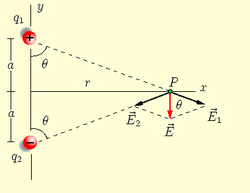
To determine the electric field which result from the dipole charges in Figure 1 that are separated by a distance 2a, we simply sum the fields from each charge individually. Note that the fields are vectors.
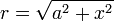
The distance of each charge (r) from the point where the electric field is measured is:
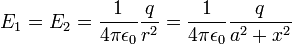
The magnitude of the electric field (E1) due to the first charge (q1) and the magnitude of the electric field (E2) due to the second charge (q2) are the same although the directions are different.
The components of the electric field along the x axis and
and have the same magnitude but opposite directions and cancel each other out.

As a result of this the horizontal components of the electric field vectors cancelling is that summing and
and reduces to summing
 and
and . Further, the magnitude of the vertical components are identical,
 . Since
 finding the vertical component reduces to:
 or:
or:
But we also know that:

So we can substitute this into the equation for which yields:

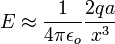
In the region distant from the dipole x is much greater than a (x>>a). This is commonly referred to as the "far field" region. We can find how the field behaves in the far field region by factoring out x.

By inspection we can conclude that when x>>a then this approaches
An important question for some analyses might be: over what range is the far field approximation valid? We can find out by using a binomial expansion (review of binomial expansion immediately below this section if you need it).
Where we will expand

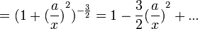
If you want to use the approximation only when it introduces an error less than 1%, then - since the first term is unity, you want the second term to be less than 1/100th of unity, or:

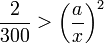


So if x is 12.3 times larger than a, this approximation is valid within 1%.
Review of the binomial expansion:


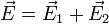
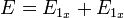
The net electric field is the sum of the contributions to the electric field from the dipole charges.
The first thing one always should do when solving a problem is to consider what you know by simple inspection. In this case the magnitude and layout of the charges tells use several things. Since they are equal and we know that the electric field from a point charge falls off as 1 over r2then we know that the nearest charge will always dominate. Further we also know that along the axis that we're calculating the electric field there will be no vertical component of the electric field.

So now we will calculate the magnitude of the electric field from each in the x direction:and.

Adding the vector magnitudesand
And substituting in the equations above yields:
![E=\frac{1}{4\pi \epsilon_0} \frac{q}{{(r-a)}^2} + \frac{1}{4\pi \epsilon_0} \frac{-q}{{(r + a)}^2}= \frac{1}{4\pi \epsilon_0}\left [ \frac{q}{{(r-a)}^2}- \frac{q}{{(r + a)}^2}\right ]=\frac{1}{4\pi \epsilon_0}\ 4aq\ \frac{r}{{(r^2 - a^2)}^2}](http://upload.wikimedia.org/math/9/6/0/96047f3dc5cb3656346fb8c6f5d2e3f3.png)
The quantity 2qa is defined as the dipole moment (p) and so we can substitute:

With that substitution we now get:
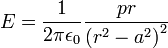
Consider the far field case (i.e., the case where >>
>> )
)
Then one can see that >>
>> and that
 approaches, which allows us to simplify the equation in the far field.

Note that one can use the binomial theorem just as in the section above to find out where this far field approximation (x>>a) is valid.
Now that you've solved for two special cases and determined that the dipole field falls off as at great distances (referred to as the far field), it is instructive to find the field's behavior off the axis.
Consider the case of an electric dipole's field at a point with the coordinates
 as represented in the figure. Note that we can represent the coordinates either as Cartesian, or as cylindrical.


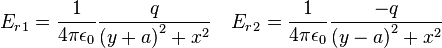
In Cartesian coordinates the electric field at any point in the plane from each charge can be found as follows:
We can apply the principle of superposition and add the fields from each of the charges, remembering that they are vectors so that the vertical components add to vertical and horizontal add to horizontal.
First finding the horizontal coordinates labeled as :
:
![{{E_r}_1}_x= \frac{1}{4\pi\epsilon_0}\frac{+q}{{(y+a)}^2+x^2}\cos\alpha=\frac{1}{4\pi\epsilon_0}\frac{+q}{{(y+a)}^2+x^2}\frac{y+a}{\sqrt{{(y+a)}^2+x^2}}=\frac{1}{4\pi\epsilon_0}\frac{+q(y+a)}{{\left [ {(y+a)}^2+x^2\right ]}^{\frac{3}{2}}}](http://upload.wikimedia.org/math/a/1/0/a10915177ee8ee812486e1c19629300f.png)
![{{E_r}_2}_x= \frac{1}{4\pi\epsilon_0}\frac{-q}{{(y-a)}^2+x^2}\cos\beta=\frac{1}{4\pi\epsilon_0}\frac{-q}{{(y-a)}^2+x^2}\frac{y-a}{\sqrt{{y-a)}^2+x^2}}=\frac{1}{4\pi\epsilon_0}\frac{-q(y-a)}{{\left [ {(y-a)}^2+x^2\right ]}^{\frac{3}{2}}}](http://upload.wikimedia.org/math/d/9/c/d9c9c9f6d3227a1b55ccc56d469aab4c.png)
Next finding the vertical components for each of the two charges labeled as we obtain:
![{{E_r}_1}_y= \frac{1}{4\pi\epsilon_0}\frac{q}{{(y+a)}^2+x^2}\sin\alpha=\frac{1}{4\pi\epsilon_0}\frac{q}{{(y+a)}^2+x^2}\frac{x}{\sqrt{{(y+a)}^2+x^2}}=\frac{1}{4\pi\epsilon_0}\frac{qx}{{\left [ {(y+a)}^2+x^2\right ]}^{\frac{3}{2}}}](http://upload.wikimedia.org/math/b/0/9/b0962381755fa9f9a776fa456da3632c.png)
![{{E_r}_2}_y= \frac{1}{4\pi\epsilon_0}\frac{-q}{{(y-a)}^2+x^2}\sin\beta=\frac{1}{4\pi\epsilon_0}\frac{-q}{{(y-a)}^2+x^2}\frac{x}{\sqrt{{y-a)}^2+x^2}}=\frac{1}{4\pi\epsilon_0}\frac{-qx}{{\left [ {(y-a)}^2+x^2\right ]}^{\frac{3}{2}}}](http://upload.wikimedia.org/math/c/6/2/c6264cc120cc04aee4cd8fe54c9fc1c5.png)
Summing the horizontal components yields:
![E_x=\frac{1}{4\pi\epsilon_0}q \left \lbrack \frac{y+a} {{\left [{(y+a)}^2+x^2 \right ] }^{\frac{3}{2}}}-\frac{y-a} {{\left [{(y-a)}^2+x^2 \right ] }^{\frac{3}{2}}}\right \rbrack
=\frac{2qa}{4\pi\epsilon_0} \left \lbrack \frac{1} {{\left [{(y+a)}^2+x^2 \right ] }^{\frac{3}{2}}}\right \rbrack](http://upload.wikimedia.org/math/1/3/3/1333ab8d0d77f56ada0e3ddc7a53ab82.png)
And for large r (either large x, large y, or their combination) this becomes:

Summing the vertical components yields:
![E_y=\frac{1}{4\pi\epsilon_0}q \left \lbrack \frac{x} {{\left [{(y+a)}^2+x^2 \right ] }^{\frac{3}{2}}}-\frac{x} {{\left [{(y-a)}^2+x^2 \right ] }^{\frac{3}{2}}}\right \rbrack](http://upload.wikimedia.org/math/b/2/4/b24cfa83fee57a042a26f2e146cd8630.png)

Last Activity: 3 Years ago
Last Activity: 4 Years ago
Last Activity: 4 Years ago
Last Activity: 4 Years ago