Statistics

• Facts, observations and information that come from investigations are termed as data. Generally there are three types of data:

• Ungrouped data, raw data or individual series

• Discrete frequency or ungrouped data

• Continuous frequency or grouped data

• Measures of central value give rough idea about where data points are centered.

• Mean, mode and median are three measures of central tendency.

• Mean is defined as the average of a distribution and is equal to ΣX/N.

• Mean can be calculated for various distributions like:

?

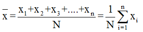
• Arithmetic mean of individual series (ungrouped data): If the series in this case be x₁, x₂, … x_n then the arithmetic mean is given by

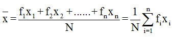
• Arithmetic mean for discrete frequency distribution: If the terms of series be x₁, x₂, … x_n and the corresponding frequencies be f₁, f₂, … , f_n then the arithmetic mean is given by 

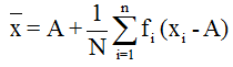
• Arithmetic mean for grouped or continuous frequency distribution: If A is the assumed mean, f the frequency and x – A = deviation of each item from the assumed mean then the arithmetic mean is given by 

• Combined Arithmetic Mean: If  (i = 1, 2, …... , k) are the means of k- component series of sizes n_i (i = 1, 2, … ,k) respectively, then the mean  of the composite series obtained on combining the component series is given by the formula  

• Weighted Arithmetic Mean: Weighted arithmetic mean refers to the arithmetic mean calculated after assigning weights to different values of variable. It is suitable where the relative importance of different items of variable is not same. It is given by

         ?

• If each of the value of a variable X is increased or decreased by some constant k then the arithmetic mean is also increased or decreased by k.

• If each of the value of a variable X is multiplied or divided by some constant k then the arithmetic mean is also multiplied or divided by k.

• Median is the score that divides the distribution into halves, half of the scores are above the median and half are below it when the data is arranged in numerical order.

• Individual series: In order to compute the median, follow the following steps:

• Arrange the data in ascending or descending order. Let n be the number of observations.

• If n is odd, Median = value of (n+1/2)th item.

• If n is even, Median = ½ [ value of (n/2)th item + value of (n/2 + 1)th item]

• Discrete series: In order to compute the median, follow the following steps:

• Arrange the data in ascending or descending order. 

• Compute the cumulative frequencies

• Median = (n/2 + 1)th item, where n is the cumulative frequency.

• Grouped or continuous distribution: In this case, the formula is given by 

           where, l = Lower limit of the median class

           f = frequency of the median class

          N = the sum of all frequencies

           i = The width of the median class 

          C = The cumulative frequency of the class preceding the median class

• Quartile: As median divides a distribution into two parts, similarly the quartiles, quantiles, deciles and percentiles divide the distribution into 4, 5, 10 and 100 equal parts.

• The jth quartile is given by

• Mode is the most frequent score in the distribution. 

• If a distribution has one mode, it is termed to be unimodal, distribution with two modes is bimodal and it is termed to be multimodal if it has more than two modes.

• Mode for continuous series: 

           where, l₁ = Lower limit of the modal class

           f₁ = frequency of the modal class

           f₀ = frequency of the class preceding the modal class

           f₂ = frequency of the class succeeding the modal class

           i = The size of the modal class 

• Symmetric distribution: A distribution is a symmetric distribution if the values of mean, mode and median coincide. In a symmetric distribution, frequencies are symmetrically distributed on both sides of the centre point of the frequency curve.

?

• A distribution which is not symmetric is called a skewed distribution.

• Empirical relation:

          Mode = 3 median – 2 mean

• A distribution is said to be positively skewed when it has a tail extending out to the right.

• The following figure illustrates the positively skewed distribution wherein mean is greater than the median and so we have the relation

          Mean > Median > Mode

• A negatively skewed distribution has an extended tail pointing to the left and reflects bunching of numbers in the upper part of the distribution with fewer scores at the lower end of the measurement scale.

• The figure below illustrates negatively skewed distribution in which Mean < Median < Mode

• Coefficient of skewness = (mean – mode)/σ

• Measures of spread/ dispersion/ variability provide information about the degree to which individual scores are clustered about or deviate from the average value in a distribution. 

• There are four measures of dispersion:

• Range is the difference between the highest and lowest score in the distribution. Coefficient of range = (L – S)/(L + S).

• The arithmetic average of the deviations from the mean, median or mode is called as mean deviation.

• Mean deviation from ungrouped data:

,

where N is the number of terms.

• Mean deviation from continuous sereis:

where N = summation of all frequencies.

• The variance is a measure based on the deviations of individual scores from the mean.

• Variance of individual observations:

          If x₁, x₂, …. , x_n are n values of a variable x, then

• Variance of discrete frequency distribution:

If x₁, x₂, …. , x_n are n values of a variable x with corresponding frequencies as f₁, f₂, ….. , f_n, then  

• Variance of a grouped or continuous frequency distribution:

• Properties of variance:

• ?If x₁, x₂, …. , x_n be n values of a variable X. If these values are changed to x₁ + a, x₂ + a, …. ….. , x_n + a, where a ∈ R, then the variance remains unchanged.

• ?If x₁, x₂, …. , x_n be n values of a variable X and let ‘a’ be a non-zero real number. Then the variance of the observations ax₁, ax₂, …. ….. , ax_n is a² Var(X).

• The positive square root of variance is termed as the standard deviation.

• If there are two sets of observations containing n₁ and n₂ items with means as m₁ and m₂ and standard deviations σ₁ and σ₂, then combined mean m is

            where d₁ = m – m₁ and d₂ = m - m₂.

• The measure of variability which is independent of units is called coefficient of variation. The coefficient of variation is given by

           where σ and are the standard deviation and mean of the data.

• A graph which displays the data by using vertical bars of various heights to represent frequencies is called a histogram. The horizontal axis can be either the class boundaries, the class marks or  the class limits.

• A frequency polygon is basically a line graph in which the frequency is placed along the vertical axis and the class mid-points are placed along the horizontal axis. These points are connected with lines.

• A frequency polygon of the cumulative frequency or the relative cumulative frequency is termed as ogive. The vertical axis represent the cumulative or the relative cumulative frequency while the horizontal axis represent the class boundaries.

• The graph of the ogive always starts at zero at the lowest class boundary and ends up at either the total frequency (for a cumulative frequency) or 1 (for relative cumulative frequency).