For projectile motion I recommend to see my earlier post on this .
Foe circular motion , u must understand the vector naature of the motion .. how it changes the direction .
Please see the derivation of circular motion in HC Verma .
If you approach circular motion problem in proper vectror notation .. its not that tough .
Non-uniform circular motion
Consider an object which executes non-uniform circular motion, as shown in Fig. 61. Suppose that the motion is confined to a 2-dimensional plane. We can specify the instantaneous position of the object in terms of its polar coordinates  and
and  . Here, is the radial distance of the object from the origin, whereas is the angular bearing of the object from the origin, measured with respect to some arbitrarily chosen direction. We imagine that both and are changing in time. As an example of non-uniform circular motion, consider the motion of the Earth around the Sun. Suppose that the origin of our coordinate system corresponds to the position of the Sun. As the Earth rotates, its angular bearing , relative to the Sun, obviously changes in time. However, since the Earth's orbit is slightly elliptical, its radial distance from the Sun also varies in time. Moreover, as the Earth moves closer to the Sun, its rate of rotation speeds up, and vice versa. Hence, the rate of change of with time is non-uniform.
Figure 61: Polar coordinates.
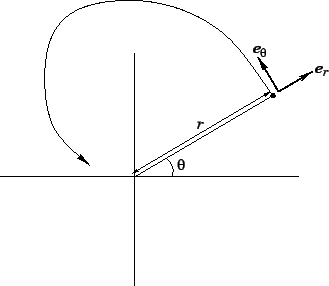 |
Let us define two unit vectors,  and
and  . Incidentally, a unit vector simply a vector whose length is unity. As shown in Fig. 61, the radial unit vector always points from the origin to the instantaneous position of the object. Moreover, the tangential unit vector is always normal to , in the direction of increasing . The position vector
  of the object can be written
 |
(270) |
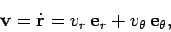
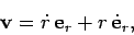
In other words, vector points in the same direction as the radial unit vector , and is of length . We can write the object's velocity in the form
 |
(271) |
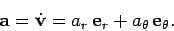
whereas the acceleration is written
 |
(272) |
Here,  is termed the object's radial velocity, whilst
  is termed the tangential velocity. Likewise,
  is the radial acceleration, and
  is the tangential acceleration. But, how do we express these quantities in terms of the object's polar coordinates and ? It turns out that this is a far from straightforward task. For instance, if we simply differentiate Eq. (270) with respect to time, we obtain
 |
(273) |
where  is the time derivative of the radial unit vector--this quantity is non-zero because changes direction as the object moves. Unfortunately, it is not entirely clear how to evaluate . In the following, we outline a famous trick for calculating , , etc. without ever having to evaluate the time derivatives of the unit vectors and .
Consider a general complex number,
 |
(274) |
where  and
and  are real, and
  is the square root of
  (i.e.,
  ). Here, is the real part of
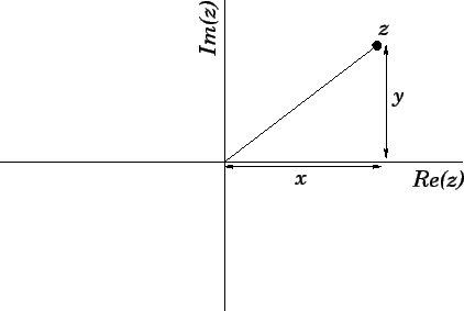
  , whereas is the imaginary part. We can visualize as a point in the so-called complex plane: i.e., a 2-dimensional plane in which the real parts of complex numbers are plotted along one Cartesian axis, whereas the corresponding imaginary parts are plotted along the other axis. Thus, the coordinates of in the complex plane are simply (, ). See Fig. 62. In other words, we can use a complex number to represent a position vector in a 2-dimensional plane. Note that the length of the vector is equal to the modulus of the corresponding complex number. Incidentally, the modulus of
  is defined
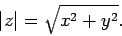 |
(275) |
Figure 62: Representation of a complex number in the complex plane.
 |
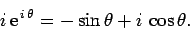
Consider the complex number  , where is real. A famous result in complex analysis--known as de Moivre's theorem--allows us to split this number into its real and imaginary components:
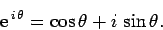 |
(276) |
Now, as we have just discussed, we can think of as representing a vector in the complex plane: the real and imaginary parts of form the coordinates of the head of the vector, whereas the tail of the vector corresponds to the origin. What are the properties of this vector? Well, the length of the vector is given by
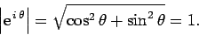 |
(277) |
In other words, represents a unit vector. In fact, it is clear from Fig. 63 that represents the radial unit vector for an object whose angular polar coordinate (measured anti-clockwise from the real axis) is . Can we also find a complex representation of the corresponding tangential unit vector ? Actually, we can. The complex number  can be written
 |
(278) |
Here, we have just multiplied Eq. (276) by , making use of the fact that . This number again represents a unit vector, since
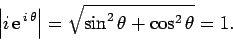 |
(279) |
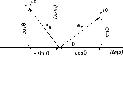
Moreover, as is clear from Fig. 63, this vector is normal to , in the direction of increasing . In other words, represents the tangential unit vector .
Figure 63: Representation of the unit vectors  and
and  in the complex plane.
 |
Consider an object executing non-uniform circular motion in the complex plane. By analogy with Eq. (270), we can represent the instantaneous position vector of this object via the complex number
 |
(280) |
Here,  is the object's radial distance from the origin, whereas
  is its angular bearing relative to the real axis. Note that, in the above formula, we are using to represent the radial unit vector . Now, if represents the position vector of the object, then
  must represent the object's velocity vector. Differentiating Eq. (280) with respect to time, using the standard rules of calculus, we obtain
 |
(281) |
Comparing with Eq. (271), recalling that represents and represents , we obtain
where  is the object's instantaneous angular velocity. Thus, as desired, we have obtained expressions for the radial and tangential velocities of the object in terms of its polar coordinates, and . We can go further. Let us differentiate
  with respect to time, in order to obtain a complex number representing the object's vector acceleration. Again, using the standard rules of calculus, we obtain
 |
(284) |
Comparing with Eq. (272), recalling that represents and represents , we obtain
Thus, we now have expressions for the object's radial and tangential accelerations in terms of and . The beauty of this derivation is that the complex analysis has automatically taken care of the fact that the unit vectors and change direction as the object moves.
Let us now consider the commonly occurring special case in which an object executes a circular orbit at fixed radius, but varying angular velocity. Since the radius is fixed, it follows that  . According to Eqs. (282) and (283), the radial velocity of the object is zero, and the tangential velocity takes the form
 |
(287) |
Note that the above equation is exactly the same as Eq. (250)--the only difference is that we have now proved that this relation holds for non-uniform, as well as uniform, circular motion. According to Eq. (285), the radial acceleration is given by
 |
(288) |
The minus sign indicates that this acceleration is directed towards the centre of the circle. Of course, the above equation is equivalent to Eq. (259)--the only difference is that we have now proved that this relation holds for non-uniform, as well as uniform, circular motion. Finally, according to Eq. (286), the tangential acceleration takes the form
 |
(289) |
The existence of a non-zero tangential acceleration (in the former case) is the one difference between non-uniform and uniform circular motion (at constant radius).


